
Intro to Multilevel Analyses
The term ‘multilevel’ refers to a hierarchical or nested data structure, usually subjects within organizational groups, but the nesting may also consist of repeated measures within subjects, or respondents within clusters, as in cluster sampling. The expression multilevel model is used as a generic term for all models for nested data. Multilevel analysis is used to examine relations between variables measured at different levels of the multilevel data structure. This book presents two types of multilevel models in detail: the multilevel regression model and the multilevel structural equation model. Although multilevel analysis is used in many research fields, the examples in this book are mainly from the social and behavioral sciences. In the past decades, multilevel analysis software has become available that is both powerful and accessible, either as special packages or as part of a general software package. In addition, several handbooks have been published, including the earlier editions of this book. The view of ‘multilevel analysis’ applying to individuals nested within groups has changed to a view that multilevel models and analysis software offer a very flexible way to model complex data. Thus, multilevel modeling has contributed to the analysis of traditional individuals within groups data, repeated measures and longitudinal data, sociometric modeling, twin studies, meta-analysis and analysis of cluster randomized trials. This book treats two classes of multilevel models: multilevel regression models, and multilevel structural equation models (MSEM). A tutorial on how to do a multilevel analysis with cross-level interaction in HLM has now also been uploaded here.
Conceptually, it is useful to view the multilevel regression model as a hierarchical system of regression equations. For example, assume that we have data from J classes, with a different number of pupils nj in each class. On the pupil level, we have the outcome variable ‘popularity’ (Y), measured by a self-rating scale that ranges from 0 (very unpopular) to 10 (very popular). We have two explanatory variables on the pupil level: pupil gender (X1: 0=boy, 1=girl) and pupil extraversion (X2, measured on a selfrating scale ranging from 1–10), and one class level explanatory variable teacher experience (Z: in years, ranging from 2–25). There are data on 2000 pupils in 100 classes, so the average class size is 20 pupils. To analyze these data, we can set up separate regression equations in each class to predict the outcome variable Y using the explanatory variables X as follows:
Yij=β0j+ β1j*X1ij+β2j*X2ij+eij
or
popularityij=β0j+ β1j*genderij+β2j*extraversionij+eij
In this regression equation, β0j is the intercept, β1j is the regression coefficient (regression slope) for the dichotomous explanatory variable gender (i.e., the difference between boys and girls), β2j is the regression coefficient (slope) for the continuous explanatory variable extraversion, and eij is the usual residual error term. The subscript j is for the classes (j=1…J) and the subscript i is for individual pupils (i=1…nj). The difference with the usual regression model is that we assume that each class has a different intercept coefficient β0j, and different slope coefficients β1j and β2j. This is indicated in the equation attaching a subscript j to the regression coefficients. The residual errors eij are assumed to have a mean of zero, and a variance to be estimated. Most multilevel software assumes that the variance of the residual errors is the same in all classes. Different authors (cf. Goldstein, 2011; Raudenbush & Bryk, 2002) use different systems of notation. This book uses σe2 to denote the variance of the lowest level residual errors. 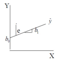
The figure to the left shows a single level regression line for a dependent variable Y regressed on a single an explanatory variable X. The regression line represents the predicted values ŷ for Y, the regression coefficient b0 is the intercept, the predicted value for Y if X=0. The regression slope b1 indicates the predicted increase in Y if X increases by one unit.
Since in multilevel regression the intercept and slope coefficients vary across the classes, they are often referred to as random coefficients. Of course, we hope that this variation is not totally random, so we can explain at least some of the variation by introducing higher-level variables. Generally, we do not expect to explain all variation, so there will be some unexplained residual variation. In our example, the specific values for the intercept and the slope coefficients are a class characteristic. In general, a class with a high intercept is predicted to have more popular pupils than a class with a low value for the intercept. Since the model contains a dummy variable for gender, the value of the intercept reflects the predicted value for the boys (who are coded as zero). Varying intercepts shift the average value for the entire class, both boys and girls. Differences in the slope coefficient for gender or extraversion indicate that the relationship between the pupils’ gender or extraversion and their predicted popularity is not the same in all classes. Some classes may have a high value for the slope coefficient of gender; in these classes, the difference between boys and girls is relatively large. Other classes may have a low value for the slope coefficient of gender; in these classes, gender has a small effect on the popularity, which means that the difference between boys and girls is small. Variance in the slope for pupil extraversion is interpreted in a similar way; in classes with a large coefficient for the extraversion slope, pupil extraversion has a large impact on their popularity, and vice versa.
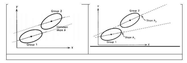
The figure to the right presents an example with two groups. The panel on the left portrays two groups with no slope variation, and as a result the two slopes are parallel. The intercepts for both groups are different. The panel on the right portrays two groups with different slopes, or slope variation. Note that variation in slopes also has an effect on the difference between the intercepts! Across all classes, the regression coefficients β0j, … β2j are assumed to have a multivariate normal distribution. The next step in the hierarchical regression model is to explain the variation of the regression coefficients β0j, … β2j by introducing explanatory variables at the class level, for the intercept:
β0j=ϒ00+ ϒ01Zj+u0j
and for the slopes:
β1j=ϒ10+ ϒ11Zj+u1j
β2j=ϒ20+ ϒ21Zj+u2j
the equation for the intercept predicts the average popularity in a class (the intercept β0j) by the teacher’s experience (Z). Thus, if ϒ01 is positive, the average popularity is higher in classes with a more experienced teacher. Conversely, if ϒ01 is negative, the average popularity is lower in classes with a more experienced teacher. The interpretation of the equations of the slopes is a bit more complicated. The first equation states that the relationship, as expressed by the slope coefficient β1j, between the popularity (Y) and the gender (X) of the pupil, depends upon the amount of experience of the teacher (Z). If ϒ11 is positive, the gender effect on popularity is larger with experienced teachers. Conversely, if ϒ11 is negative, the gender effect on popularity is smaller with more experienced teachers. Similarly, the second equation states, if ϒ21 is positive, that the effect of extraversion is larger in classes with an experienced teacher. Thus, the amount of experience of the teacher acts as a moderator variable for the relationship between popularity and gender or extraversion; this relationship varies according to the value of the moderator variable. The u-terms u0j, u1j and u2j in the equations are (random) residual error terms at the class level. Note that in the above equations the regression coefficients ϒ are not assumed to vary across classes. They therefore have no subscript j to indicate to which class they belong. Because they apply to all classes, they are referred to as fixed coefficients. All between-class variation left in the β coefficients, after predicting these with the class variable Zj, is assumed to be residual error variation. This is captured by the residual error terms uj, which do have subscripts j to indicate to which class they belong.
Our model with two pupil level and one class level explanatory variables can be written as a single complex regression equation by substituting equations 2.3 and 2.4 into equation 2.1. Substitution and rearranging terms gives:
Yij=ϒ00+ ϒ10X1ij+ ϒ20X2ij+ϒ01Zj + ϒ11X1ijZj+ ϒ21X2ijZj + u1jX1ij+u2jX2ij +u0j+eij
or
popularityij=ϒ00+ ϒ10*genderij+ ϒ20*extraversionij+ϒ01*experiencej + ϒ11*genderij*experiencej+
ϒ21*extraversionij*experiencej + u1j*genderij+u2j*extraversionij +u0j+eij
For a more thorough introduction and some useful examples please read the second chapter of the book on ‘Basic Two-Level Regression Model’ which can be downloaded here.